Computational design strategy
Assembly backbone design with RFdiffusion
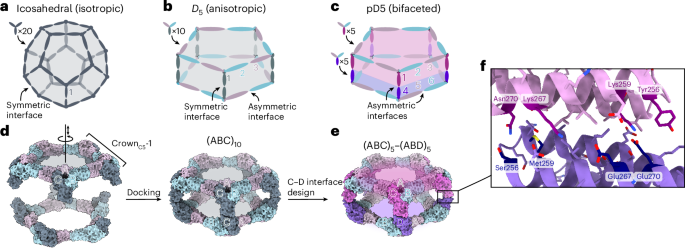
We used RFdiffusion to design symmetric homo-oligomers that rigidly hold bonding motifs such that they exactly match the presentation orientation of existing binding partners (Extended Data Fig. 1). In a typical input preparation, we first create a virtual building block C3-AB′, by symmetrically arranging fragments of the complementary binding partners for an existing cyclic oligomer C3-A. The outward-facing virtual building block C3-AB′ has a central cavity, but contains geometric constraints. Next, we symmetrically arrange C3 assemblies to sample rotations and translations along their new symmetry axes. New oligomeric binding partners were then isolated and created through symmetric RFdiffusion. For constructs generated using WORMS (for example, for pyramidal symmetry), these spatial configurations between the two C3 complexes were checked to see whether rigid fusions could connect the top and bottom subunits via a simple helix alignment. For constructs generated using RFdiffusion (dihedral symmetry), symmetric denoising was performed, to connect the top and bottom subunits with new C2-symmetric interfaces.
Backbone generation with WORMS
A library of cyclic oligomer scaffolds (C2, C3 and C4) from crystal structures deposited in the Protein Data Bank18,36,37,38,39 (http://www.rcsb.org/pdb/) and from previous de novo designs were used as the input scaffolds. To enable the generation of a diverse range of architectures, we guide the WORMS software with a configuration file to truncate inputs from the structural database and exhaustively for fusible bridging elements. The default WORMS settings were used, except that the ‘tolerance’ parameter was set to 0.1 from 0.25 to reduce closing error (‘tolerance’ defines the permitted deviation of the final segment from its targeted position within the structure). The number of backbone fusion outputs produced depends on the allowed fusion points and tolerance parameter, as the design space expands exponentially with the number of segments being fused.
Sequence design with ProteinMPNN
We performed three cycles of ProteinMPNN40 and Rosetta41 FastRelax to design sequences for backbones generated from RFdiffusion or WORMS protocol. For homomeric oligomer designs, it is possible to restrict the sequences to be identical between the structural elements where that is desired, using the –tied_positions argument as described.
In silico filtering
AlphaFold2 was used to assess whether our designed sequences will fold or assemble as intended. We primarily used the prediction results from Model 4 as it usually provided the highest-confidence predictions for all α-helical proteins. The computational metrics23 filtering cut-offs were set to predicted local-distance difference test (pLDDT) score > 90, predicted template modelling (pTM score) > 0.80 and Cα root mean square deviation of less than 1.5 Å or 2.0 Å compared with the ideal design model.
RPXDock cage docking and design
Homotrimeric and heterotrimeric rings were computationally docked to create backbone configuration for the O3 and D4 cages, respectively. The O3-symmetric cage was adapted to a three-component D4-symmetric assembly using RFdiffusion and interface exchange (Extended Data Fig. 2). The sequence of cage-contacting interfaces were redesigned by ProteinMPNN, following a rigorous Rosetta filtering41 process based on several metrics, including a methionine count of ≤5, shape complementarity of >0.6, change in Gibbs free energy (ddG) of less than –20 kcal mol−1, solvent-accessible surface area of <1,600, clash check of ≤2 and unsatisfied hydrogen bonds of ≤2. To improve the cage yield and reduce aggregation propensity, we further optimized their sequences using ProteinMPNN and filtered designs based on the change in spatial aggregation propensity (SAP) score of <30.
Protein expression and purification
Synthetic genes from computationally filtered designs were acquired from IDT and cloned into the pET29b+ vector using NdeI and XhoI restriction sites. These designs were expressed in BL21* (DE3) E. coli-competent cells using a bicistronic system with a C-terminal polyhistidine tag. For protein expression, transformants were cultured in 50-ml Terrific Broth supplemented with 200 mg l−1 kanamycin and induced for 24 h at 37 °C under a T7 promoter. Cells were harvested by centrifugation, resuspended in Tris-buffered saline and lysed with 5 min of sonication. The lysates were then subjected to nickel affinity chromatography, washed with ten-column volumes of 40-mM imidazole and 500-mM NaCl, and eluted with 400-mM imidazole and 75-mM NaCl. Successful complex formation was confirmed by the presence of both oligomers on sodium dodecyl sulfate–polyacrylamide gel electrophoresis following Ni-NTA pulldown. Proteins of the correct molecular weights were further analysed by electron microscopy. Selected designs were scaled up to 0.5 l for additional expression and purification under the same conditions. The in vitro assembly of complexes was achieved by mixing individually purified components at equimolar ratios, with 18 assemblies displaying SEC profiles consistent with the designed oligomeric states.
nsEM
Cage fractions obtained from the SEC traces or by in vitro mixing were diluted to a concentration of 0.5 µM (monomer component) for characterization by nsEM. A 6-µl sample of each fraction was placed on glow-discharged, formvar/carbon-supported 400-mesh copper grids (Ted Pella) and allowed to adsorb for over 2 min. Each grid was blotted and stained with 6 µl of 2% uranyl formate, blotted again and restrained with an additional 6 µl of uranyl formate for 20 s before the final blotting step. Imaging was performed using a Talos L120C transmission electron microscope operating at 120 kV.
All the nsEM datasets were processed using CryoSparc software. Micrographs were uploaded to the CryoSparc web server, and the contrast transfer function was corrected. Approximately 200 particles were manually selected and subjected to 2D classification. Selected classes from this initial classification served as templates for automated particle picking across all the micrographs. Subsequently, the particles were classified into 50 classes through 20 iterations of 2D classification. Particles from the selected classes were utilized to construct an ab initio model. Initial models were further refined using C1 symmetry and the corresponding T/O-symmetry adjustments.
Cryo-EM sample preparation, data collection and processing
T33-549 cage
T33-549 solution (8.5 mg ml−1 in 25 mM of Tris (pH 8) with 300 mM of NaCl) was diluted 1:9 in a sample buffer, and then, the grids were immediately prepared using Vitrobot Mark IV in which the chamber was maintained at 22 °C and 100% humidity. Then, 3.5 µl of diluted T33-549 (final concentration, ~0.9 mg ml−1) was applied to the glow-discharged surface of grids (QUANTIFOIL R 2/2 on Cu 300 mesh + 2-nm C) and then immediately plunged into liquid ethane after blotting for 4 s with a blot force of 0. Grids were first screened at the NYU Cryo-Electron Microscopy Laboratory on a Talos Arctica microscope operated at 200 kV and equipped with an energy filter and Gatan K3 camera. Data were then collected at the National Center for Cryo-EM Access and Training (NCCAT) at the New York Structural Biology Center on a Titan Krios microscope operated at 300 kV with a Gatan K3 camera. Furthermore, 12,276 videos were collected, and all data acquisition was controlled using Leginon42. The data acquisition parameters are shown in Supplementary Table 4.
The data processing workflow is described in Supplementary Fig. 2. Videos were imported into CryoSPARC43 for processing and split into 13 subsets during the initial processing steps. After patch motion correction and contrast transfer function estimation, images were curated, leading to the removal of 696 micrographs. Another 253 micrographs were randomly selected to generate templates using both manual picking and blob picker, and the picked particles were fed into 2D classification jobs. The resulting templates (14,616 particles from the 5 best classes) were used to train Topaz (conv127)44, which was then used to pick all micrographs. The resulting 4,841,024 particles were extracted at 4.94 Å pixel−1 and two rounds of 2D classification were carried out, followed by the removal of duplicate particles for each of the 13 subsets of micrographs. The resulting 1,058,870 particles were then grouped into three subsets for further processing. One of these groups was used to generate an ab initio model (using T symmetry). Each of the three subsets was then fed into 3D homogeneous refinement jobs, leading to ~10-Å models. After 3D heterogeneous refinement in C1 symmetry, bad classes were removed, leading to 751,758 particles among the three subsets. Particles were re-extracted at 1.24 Å pixel−1 before another round of 3D refinement without symmetry applied and another round of 3D heterogeneous refinement. The best classes of the three subsets were then merged, leading to an ~7.0-Å resolution map (C1), and two more rounds of non-uniform refinements45 were performed, leading to a resolution of 6.8 Å without symmetry (C1) and 6.1 Å with T symmetry (Supplementary Fig. 3a,b). The map using T symmetry has a sphericity46 of 0.972 (unmasked). The design model was then docked as a rigid body into the resulting map using Chimera UCSF47 (Supplementary Fig. 3c), followed by conservative real-space refinement in Phenix48 (Supplementary Fig. 3d), with constraints on the secondary structure (Supplementary Table 5).
O42-24 cage
2 µl of the cages at a concentration of 1.3 mg ml−1 in 150 mM of NaCl and 25 mM of Tris (pH 8.0) was applied to glow-discharged QUANTIFOIL R 2/2 on Cu 300-mesh grids + 2-nm C grids. The grids were plunge frozen in liquid ethane using Vitrobot Mark IV, with a wait time of 7.5 s, blot time of 0.5 s and a blot force of –1. A total of 3,196 videos were collected in the counting mode, each consisting of 75 frames, using a Titan Krios microscope operating at 300 kV and equipped with an energy filter. The pixel size was 0.84 Å, with a total dose of 61 e⁻ Å−2 per video.
All data processing was carried out using CryoSPARC v. 3.3.2 (ref. 43). Patch motion correction and patch contrast transfer function estimation were performed using default parameters. An initial set of 224,225 particles was picked using the blob picker tool, followed by extraction at a box size of 640 pixels and Fourier cropping to 320 pixels. 2D class averages were generated, and the nine best classes were low-pass filtered to 20 Å to serve as references for template-based particle picking, resulting in a refined set of 185,832 particles. These particles were re-extracted using a 640-pixel box size and Fourier cropped to 320 pixels. A subsequent 2D classification into 100 classes identified 69,634 high-quality particles, which were used for ab initio 3D reconstructions, sorted into three classes with octahedral symmetry applied. Non-uniform refinement, using the best ab initio map as the initial model and all 69,634 of the best particles from the 2D classification, yielded a final 3D map with a global resolution estimate of 8.3 Å.
SAXS data collection and pattern simulation
SAXS was performed on a Xenocs Xeuss 3.0 instrument with an X-ray energy of 8.04 keV (wavelength, 1.54 Å) using a Cu Kα microfocus source. Data were collected in three configurations: low-q (0.003–0.007 Å−1) for 18,000 s, mid-q (0.007–0.020 Å−1) for 10,000 s and high-q (0.020–0.200 Å−1) for 7,200 s. Samples were loaded in 1.5-mm-diameter thin-walled quartz capillary that were purchased from Charles Supper. Data reduction was performed by subtracting the background from another capillary with the water solvent. Data reduction and merging were performed using the XSCAT software (v2.10.3).
The simulated small-angle scattering curves of the computational models of the protein crystals were calculated by using a Monte Carlo sampling of the Debye equation. This method allows for a fast and accurate calculation of the scattering curve of large structures49,50. In short, the atomic coordinates of each atom were first extracted from the Protein Data Bank file of the protein crystal. X-ray scattering length densities51 were then assigned to each atom. Two random coordinates were then selected and the distance between these points was calculated. After sampling 10 million pairs of random coordinates, the pairwise distribution was created, which was then transformed into the scattering curve using Fourier inversion. The code and notebook used to perform this simulation is available online (https://github.com/pozzo-research-group/MC-DFM/tree/main/Notebooks).