Computational design of bifaceted protein nanomaterials

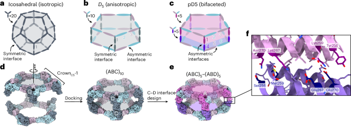
Docking

From the PDB file containing Crown_C5-1, which had its five-fold rotational symmetry axis aligned to the z axis, we removed all but three chains of one ABC heterotrimer and truncated the C component by 1–4 helices. Because RPXdock is limited to single-chain inputs, for each instance of the heterotrimer with the truncated C component, we connected amino acid residues of all the three chains of the heterotrimers into one chain and saved as a new PDB. These PDB structures were used as the input files for docking into D5_5 by restricting sampling to rotation and translation along the z axis using RPXdock⁵² (https://github.com/willsheffler/rpxdock). The top scoring and the output with the highest shape compatibility was taken for further design.

Asymmetric interface design

The design of an asymmetrical C–D interface was carried out using the deep learning-based protein sequence design software ProteinMPNN (https://github.com/dauparas/ProteinMPNN). We used ProteinMPNN without biases, ProteinMPNN with adding biases to specific amino acids per residue position and multistate ProteinMPNN. For each method, 100 sequences were designed across different temperatures (0.1, 0.2, 0.4, 0.5, 0.6, 0.8 and 1.0). In the ProteinMPNN with bias per residue position approach, we increased the likelihood of specific amino acids occupying predefined positions using a biasing script (https://github.com/dauparas/ProteinMPNN/blob/main/helper_scripts/make_bias_per_res_dict.py) with a small modification. This script normally favours certain amino acids at specific positions in one chain and disfavouring them in another chain. We modified it to apply positive biases for both chains to increase the probability of the desired amino acids being incorporated on a predefined side. Specifically, we categorized the amino acids S, T, N, Q, V, I and L as small; F, Y and W as bulky; D and E as negatively charged; and R, H and K as positively charged. We biased amino acids in three ways. In the ‘charges’ approach, we favoured positively charged amino acids on one side and negatively charged on the other side. In the ‘clashes’ approach, we favoured small amino acids on one side and bulky on the other side. In ‘charges-clashes’, we favoured positively charged and bulky amino acids on one side and negatively charged and small amino acids on the other side. Bias values of 0.1, 0.2, 0.69, 1.1 and 3.9 were used for both sides in each biasing approach, where 0.69 was for two-fold, 1.1 for three-fold and 3.9 for four-fold increase in likelihood to incorporate the desired amino acid. Multistate ProteinMPNN design was performed as previously described³⁶ using β-values of –1, –0.5 and –0.25.

Extension of the C component using RFdiffusion

Translation of the portion of (ABC)₅ cyclic assemblies was done in PyMOL Molecular Graphics System (v. 2.5.8, Schrödinger). For the full structure extension process, we reasoned that extending only one C component is sufficient, given that the C components are organized in C₅ symmetry and there are no neighbouring subunits with which extensions might clash. For easier computing and to streamline the design filtration process, only four helices of the translated portion of the C component and two isolated helices belonging to the C component were used as an input for RFdiffusion. For each extension distance value, we generated 100 backbones using RFdiffusion (https://github.com/RosettaCommons/RFdiffusion). The ranges of amino acids provided for diffusion to generate the backbones within the gaps were as follows: 50–150, 100–250, 150–350 and 250–400 residues for extensions of 25 Å, 50 Å, 75 Å and 100 Å, respectively. For the 50-Å extension with a subsequent 25° rotation, we used a range of 150–350 residues. The range of amino acids needed to fill the gaps was initially estimated visually for the 25-Å extensions, with an allowance of ±50 residues. For subsequent extensions, the range was determined based on AF2 predictions for the successful 25-Å extensions.

Reorienting N termini using RFdiffusion

To reorient the N termini, we used RFdiffusion with block adjacency⁴⁵. Briefly, we started by modifying the Protein Data Bank (PDB) structure of the ABC heterotrimer to mimic the desired structure with the reoriented N terminus. This involved deleting three loops and adding new loops and one helix of the desired length in specific locations, which we treated as separate chains. These modifications were made using PyMOL. The manipulated PDB structure was then used to create an adjacency matrix, which provided information on which helices the newly built helix (using RFdiffusion) should interact with. RFdiffusion was subsequently used to rebuild the new loops and the helix, generating 100 new heterotrimer backbones.

Construction of synthetic genes

All the synthetic genes were purchased from GenScript. They were codon optimized for expression in E. coli and cloned into pET29b+ plasmid between Ndel/Xhol sites. Only the A component had 6×His tag on the C terminus for facilitating the IMAC purification of complexes. The C and D components had mScarlet and mNeonGreen fused to the N terminus, respectively, for easier detection by SEC and SDS-PAGE gel.

Protein expression

Then, 100 ng of each plasmid obtained from GenScript was diluted in 20 µl of DNase-free water (Cytiva). Also, 0.5 µl of each plasmid was used for the transformation of 5 µl of BL21(DE3)Star E. coli expression strain (Invitrogen) according to the manufacturer’s protocol. One bacterial colony was inoculated in 5 ml of Luria Bertani medium containing 100 µg ml⁻¹ of kanamycin and grown overnight at 37 °C with shaking at 225 rpm. Then, 1 ml of the overnight culture was transferred to 50 ml of Terrific Broth II media (MP Biomedical, cat. no. MP113046052) supplemented with 100 µg ml⁻¹ of kanamycin in 250-ml flasks. Bacteria was grown at 37 °C until the optical density was 0.6–0.8, and then, the protein expression was induced by adding isopropyl β-d-1-thiogalactopyranoside, after which the temperature was decreased to 18 °C. Expression was continued for 20–24 h with shaking at 225 rpm.

IMAC

Here 50-ml cultures were harvested by centrifugation at 4,000g for 20 min at 4 °C. Pelleted bacteria were resuspended in 10 ml of lysis buffer (50 mM of Tris pH 8.0, 300 mM of NaCl, 20 mM of imidazole and 10% glycerol). Resuspensions of A, B and C or A, B and D components were mixed and 300 µl of phenylmethanesulfonyl fluoride (100 mM in 20% ethanol) was added to the mixtures. Immediately on adding phenylmethanesulfonyl fluoride, mixtures were sonicated at 65% power for 5 min, with 10 s of ON/OFF pulse. Lysed bacteria were left on ice for 30 min to allow the formation of ABC heterotrimers and (ABC)₅ or (ABD)₅ cyclic assemblies, and subsequently centrifuged at 14,000g for 30 min at 18 °C. Following centrifugation, the supernatant was kept for an additional 30 min at room temperature to ensure the proper assembly of (ABC)₅ or (ABD)₅ cyclic assemblies. Subsequently, the supernatant was applied to 1 ml of Ni-NTA resin (Qiagen) for gravity chromatography, which was pre-equilibrated with 5 ml of lysis buffer. Columns were washed with 15 ml of wash buffer (50 mM of Tris pH 8.0, 300 mM of NaCl, 40 mM of imidazole and 10% glycerol) and the protein was eluted with 1.7 ml of elution buffer (50 mM of Tris pH 8.0, 300 mM of NaCl, 300 mM of imidazole, 300 mM of EDTA and 10% glycerol). Only the last 1.3 ml of the elution was collected for further purification.

SEC

Here 1.3 ml of the sample obtained by IMAC purification was further purified using a Superose 6 10/300 Increase column (Cytiva) in SEC buffer (50 mM of Tris pH 8.0 and 300 mM of NaCl) with an ÄKTA Pure chromatography system. In addition to 280-nm absorbance, absorbance at 506 nm and 569 nm was followed. On mixing (ABC)₅ and (ABD)₅ cyclic assemblies, a second SEC purification was performed using the same buffer.

SDS-PAGE

Peak fractions of cyclic assemblies and D₅ assemblies were analysed by SDS-PAGE electrophoresis. Here 1–5 µg of target protein was resuspended in 2× Laemmli Sample Buffer (Bio-Rad) with adding 1:20 β-mercaptoethanol and 15 µl of the mixture was added onto Any kD Criterion TGX Stain-Free Protein gel (Bio-Rad). Then, 5 µl of Precision Plus Protein Unstained Protein Standards (Bio-Rad) was used and the gels were run at 150 V for ~50 min. Subsequently, the gels were stained with GelCode Blue (Thermo Fisher Scientific) and destained in water. The stained gels were imaged using a Chemidoc XRS+ (Bio-Rad).

nsEM

Here 3 µl of the SEC-purified samples with an approximate concentration of 0.05 mg ml⁻¹ was deposited on 10-nm-thick carbon-film-coated 400-mesh copper grids (Electron Microscopy Sciences, CF400-Cu-TH) that was previously glow discharged for 20 s. Subsequently, the grids were stained three times using 2% uranyl formate. Grids were screened using a 120-kV Talos L120C transmission electron microscope. For collecting large datasets to obtain 2D class averages and 3D reconstruction, E. Pluribus Unum (FEI Thermo Scientific) software (v. 2.12.1.2782REL and 3.1.0.4506REL) was used. Data processing was done using CryoSPARC v. 4.2.2, v. 4.4.0 and v. 4.4.1 (Structura Biotechnology). We initially used D₅ symmetry to generate the nsEM models, which then served as the starting point for the subsequent C₁ reconstructions. Fitting of the design models into corresponding density maps was done using ChimeraX^61,62,63.

DLS

To determine the size and uniformity of the particles, DLS measurements were performed using the sizing and polydispersity method on the Uncle instrument (Unchained Labs). Here 8.8 µl of SEC peak fractions were loaded into the provided glass cuvettes. DLS measurements were measured in triplicate at 25 °C; 10 acquisitions were done, with each measuring 10 s in length. To determine the stability of the nanoparticles, SLS and intrinsic tryptophan fluorescence (presented as the barycentric mean of the emission spectrum) were measured in triplicate at 25 °C, followed by a thermal ramp from 25 °C to 95 °C at a ramp rate of 1.0 °C min⁻¹. Protein concentration (ranging from 0.1 mg ml⁻¹ to 0.4 mg ml⁻¹) and buffer conditions were accounted for in the software. Data were processed using Uncle Analysis software (v. 6.01.0.0).

MP

All the MP measurements were carried out on a TwoMP Auto mass photometer using the AcquireMP software (v. 2024 R1.1, Refeyn). Proteins were diluted to ~20 nM at least an hour before measurement in a flat-bottom 96-well polypropylene plate (Greiner). After centring the laser over a well on a 24-well gasket on commercially precleaned slides (Refeyn), 5 µl of buffer (50 mM of Tris and 300 mM of NaCl, pH 8) was deposited into the well using the automated fluid-handling system and used for finding focus using the drop dilution method. After the focus was found, 5 µl of the sample was pipetted into the gasket well and mixed once. One-minute videos were recorded using the normal field of view. Ratiometric contrast values for individual particles in each video were measured and processed into mass distributions with DiscoverMP (v. 2024 R1) using a sample of 20 nM of β-amylase (containing monomers (56 kDa), dimers (112 kDa) and tetramers (224 kDa)) as mass standards. DiscoverMP was used to fit the Gaussian distributions to the experimental mass distributions to calculate the mean mass of the particles.

Cryo-EM sample preparation

To prepare the sample for cryo-EM, 3 µl of the construct at a concentration of 1.5 mg ml⁻¹ was pipetted onto a glow-discharged 400-mesh copper ultrathin lacey carbon grid (Electron Microscopy Sciences, LC400-Cu-CC-25). The grid was immediately vitrified by plunge freezing into liquid ethane using a FEI Vitrobot Mk. IV at 22 °C, 100% humidity, with a 7.5-s wait time and a 0.5-s blot time at –1 blot force. Subsequently, the grid was clipped and remained continuously submerged in liquid nitrogen until it was loaded onto the microscope.

Cryo-EM data processing

Using a 300-kV FEI Titan Krios device with a Gatan K3 direct electron detector and a Gatan BioQuantum energy filter, 4,871 videos were collected in SerialEM, utilizing beam shifts to collect 11 videos per stage movement at ×105,000 magnification with a pixel size of 0.843 Å pixel⁻¹. Image stacks were composed of 79 frames at an exposure rate of 0.0505 s per frame with a dose weight of 11.31 e⁻ A⁻² s⁻¹ and an exposure time of 3.997 s, resulting in a total dose of 45.21 e⁻ Å⁻². All the videos were then imported into CryoSPARC v. 4.4, where all the data processing took place. First, exposures were preprocessed using patch motion correction, patch contrast transfer function estimation and videos were curated, eliminating videos with contrast transfer function fit resolutions below 6 Å and those with average intensities above 472.77. Because of the central cavity and variable diameter of our proteins’ minor axis at different view angles, blob picking was unsuccessful. 177 particles were first manually selected, extracted to 800 pixels (952.4 Å) and classified into 2D class averages to generate templates. Two sequential rounds of template picking, extraction to 800 pixels and 2D classification into 150 classes followed, resulting in a final population of 209,004 particles. Those particles were homogeneously refined in C₅ symmetry using an ab initio volume map of this construct previously characterized by nsEM, which was low-pass filtered to 50 Å. Particles were downsampled to 400 pixels to reduce the processing bandwidth before the volume was subsequently refined using non-uniform refinement. Local contrast transfer function refinement was then performed on the particles followed by another round of non-uniform refinement. To finalize the model, one last homogeneous refinement was performed (generating our final half-maps and a global resolution of 4.30 Å), which was then sharpened using a B factor of 239.90 (derived from our homogeneous refinement) sharpened using DeepEMhancer⁶⁴ to generate our deposited Coulombic potential map.

Cryo-EM model building

To build our model, the computationally designed model was rigid-body docked into the final cryo-EM map in ChimeraX and was subsequently trimmed to PolyA in Phenix^65,66, and the backbone was relaxed into our volume map using Namdinator⁶⁷. We then manually refined the backbone using ISOLDE⁶⁸ in ChimeraX, and Coot⁶⁹. Side chains were trimmed to PolyA and a wwPDB validation service^70,71 report was generated to verify that the model’s clashscore and Ramachandran outliers were each zero (Supplementary Table 2). The final structure was deposited in the PDB and Electron Microscopy Data Bank under accession nos. 9DZE and EMD-47327, respectively.

BLI

BLI was performed on Octet R8 (Sartorius). All the biosensors were hydrated in a kinetic buffer (10 mM of HEPES pH 7.4 and 1% w/v of bovine serum albumin (BSA)). Biotinylated human IL-2Rβ (Acro Biosystems, ILB-H82E3) and human 4-1BB (Sino Biological, 10041-H27H-B) were diluted to a concentration of 2.5 μg ml⁻¹ in the kinetic buffer and loaded onto streptavidin-coated biosensors (SAForteBio). Complexes were diluted in the kinetic buffer to a concentration of 15 nM and its association was measured for 300 s, followed by a dissociation for 300 s in the kinetic buffer. Data were processed using ForteBio Data Analysis software (v. 9.0.0.10).

Flow cytometry

Here 200 μl of streptavidin-coated fluorescent Nile Red and purple particles with a nominal size of 5.0–7.9 µm (Spherotech) were washed three times in phosphate-buffered saline (PBS) containing 0.01% Tween 20 and 0.05% BSA according to the manufacturer’s protocol with spinning for 30 s at 21,000g. After washing, both particle types were resuspended in 250 μl of PBS with 0.01% Tween 20 and 0.05% BSA. Biotinylated human IL-2Rβ (Acro Biosystems, ILB-H82E3) and human 4-1BB (Sino Biological, 10041-H27H-B) were incubated with Nile Red and purple particles, respectively, at a concentration of 10 μg of receptor per 1 mg of Spherotech streptavidin particles, with gentle rotation for 30 min. The particles coated with biotinylated receptors were separated from unbound receptors by centrifugation at 21,000g for 30 s, followed by five washes in PBS with 0.01% Tween 20 and 0.05% BSA. On washing, particles were resuspended in 250 μl of PBS with 0.01% Tween 20 and 0.05% BSA. Finally, 1 μl of each particle suspension was further resuspended in 18 μl of PBS with 0.01% Tween 20 and 0.05% BSA, to which 100 μl of the sample was added. The mixture was incubated at room temperature for 30 min and colocalization events were acquired using an AttuneNXT flow cytometer (Thermo Fisher). Data files were analysed using FlowJo software (v. 10; BD Biosciences). Statistical analysis was performed using a one-way analysis of variance with Geisser–Greenhouse correction followed by Tukey’s multiple comparisons test, with individual variances computed for each comparison.

Fluorescence microscopy

Coating streptavidin-coated fluorescent Nile Red and purple particles with biotinylated human IL-2Rβ (Acro Biosystems, ILB-H82E3) and human 4-1BB (Sino Biological, 10041-H27H-B) was performed following the same procedure as the flow cytometry experiments. Here 1 μl of each particle suspension was resuspended in 18 μl of PBS containing 0.01% Tween 20 and 0.05% BSA. Then, 4 μl of this mixture was incubated with 20 μl of the sample at room temperature for 30 min. Subsequently, the mixture was placed in a glass-bottom 18-well ibidi slide and the particles were allowed to settle for 10 min before imaging. Images were acquired on an IN Cell Analyser 2500HS microscope using a Nikon Plan Apo, CFI/60 ×20 objective with a numerical aperture of 0.75. Fluorescent particles were excited using light-emitting diodes emitting at 473 nm and 575 nm each with 10-ms exposure times. Emission was collected through bandpass filters centred at 525 (±24) nm and 623 (±12) nm, respectively. Each sample was imaged in 25 separate fields of view for quantification. Briefly, quantification was carried out using a custom Python script (Python v. 3.12.8) that segmented fluorescent particles in each channel and then, using one channel as a reference, measured the distance between each identified fluorescent particle and all the fluorescent particles of the opposite colour. Only fluorescent particles with a centroid-to-centroid separation distance of less than 7.5 µm (representing roughly twice the radius of the fluorescent particle) were kept as positive hits for fluorescent particle interaction. Per-cent fluorescent particle interactions were then determined by dividing the interacting fluorescent particles by the total fluorescent particle count for each channel in each image.